Vector search is easy until you add a filter. “Find me similar documents” is a clean nearest-neighbor query; “find me similar documents where tenant = acme and lang = en” is where the standard index — HNSW — quietly falls apart. I read how Qdrant handles it at v1.18.2, commit 44ad62f, and the answer is two specific engineering moves: it estimates the filter’s cardinality to pick a search strategy, and it builds extra graph links so a filtered subgraph doesn’t disconnect. Every claim points at a line.
HNSW in thirty seconds
Qdrant’s vector index is HNSW — a hierarchical navigable small-world graph. Each point is assigned a random top level from a geometric distribution (-ln(u) * level_factor, graph_layers_builder.rs:391), so the upper layers are sparse and layer 0 is dense. A query enters at the top and greedily hops to the single best neighbor down through the sparse layers (graph_layers.rs:299), then runs an ef-width beam search on the base layer, keeping the best ef candidates in a fixed-size queue and stopping when the frontier can’t beat the ef-th best (graph_layers.rs:126). Neighbors are chosen at build time by a diversity heuristic — drop a candidate if it’s closer to an already-picked neighbor than to the point itself (links_container.rs:59) — capped at m links per node (m0 = 2m on layer 0). Defaults: m = 16, ef_construct = 100 (types.rs:1414).
Why a filter breaks it
Now add tenant = acme. You have two bad options. Post-filter: run the normal graph search, then throw away results that don’t match — but if only 1% of points are acme, the top-ef are almost all discarded and recall collapses. Pre-filter: fetch the matching set first, but a raw list of matching ids can’t exploit the graph’s structure, so you’re back to scanning. Qdrant refuses both defaults and makes a decision instead.
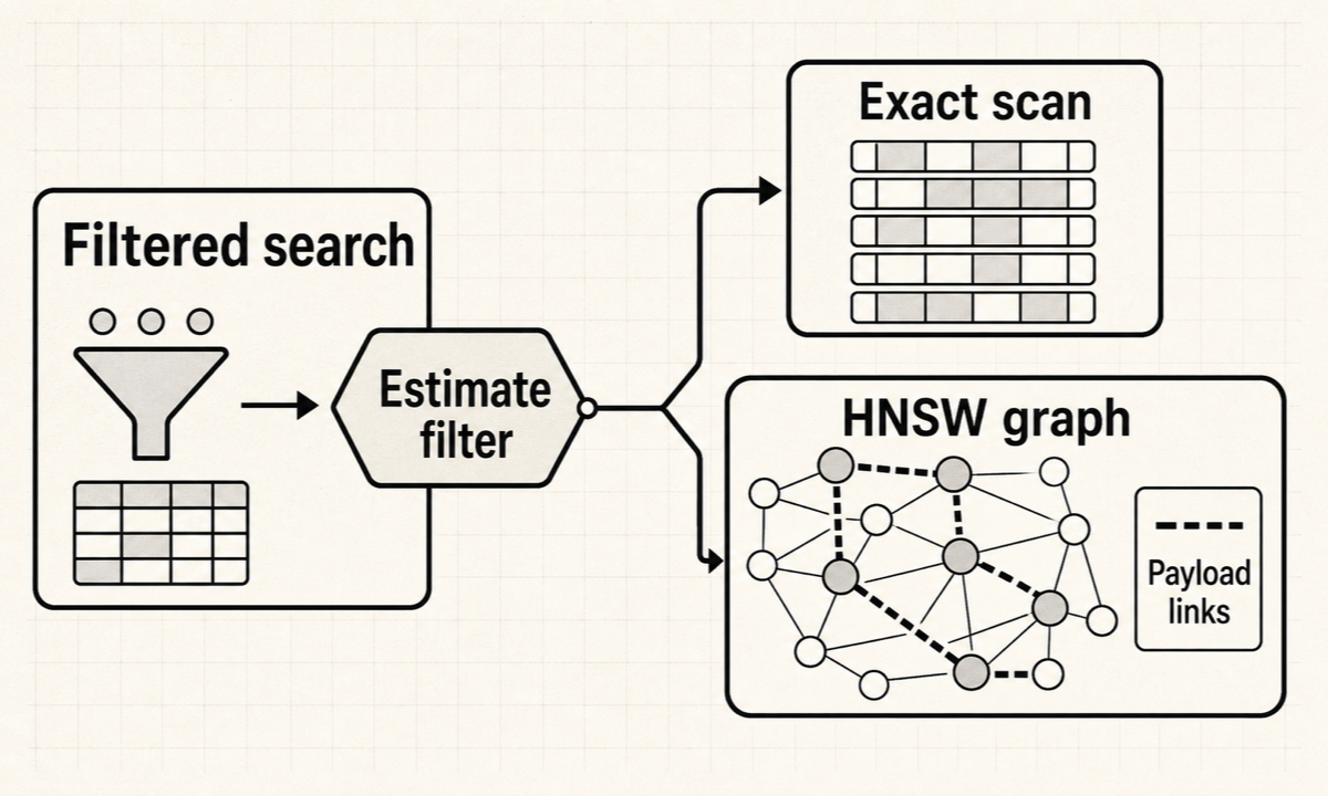
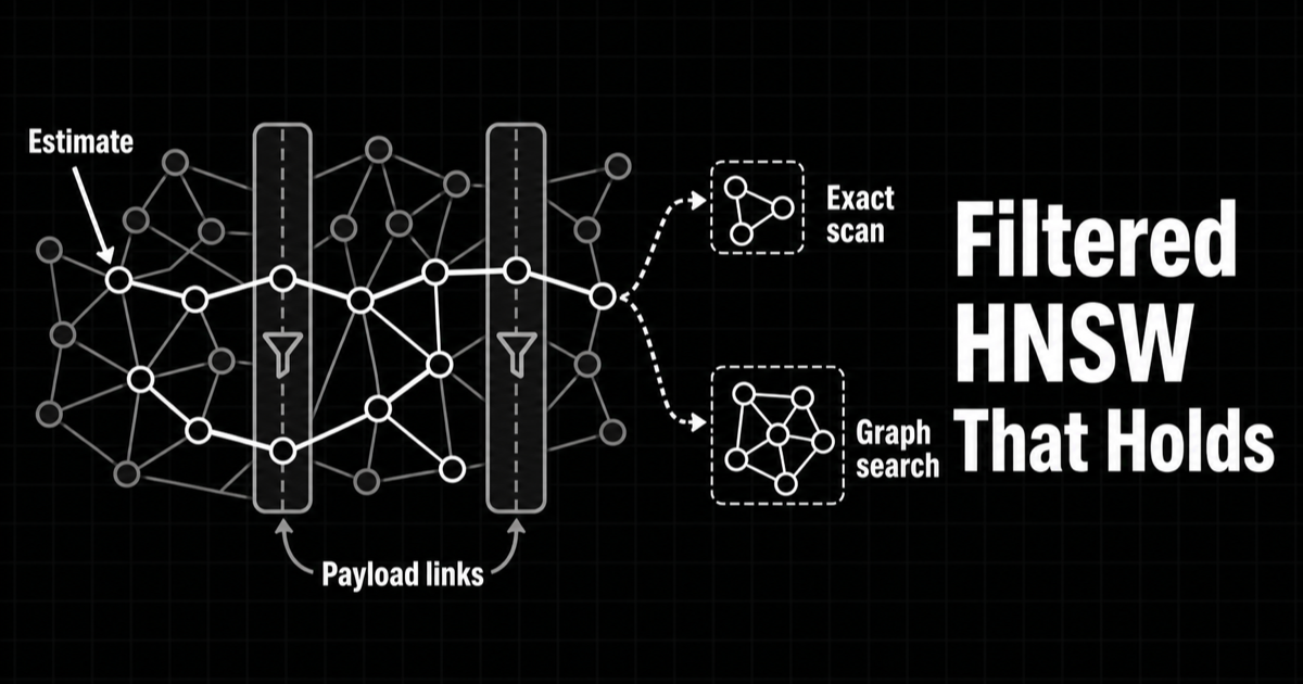
Qdrant makes the payload filter part of the search plan: estimate cardinality first, then choose exact filtered scan or graph search with payload-aware links.
Move 1: estimate the filter, then pick a strategy
Before searching, Qdrant asks the payload index how many points will this filter match? — estimate_cardinality returns a { min, exp, max } range (vector_index_impl.rs:114; for an exact keyword match the count is exact). Then it branches on the configured full_scan_threshold:
| Estimated cardinality | Strategy | Why |
|---|---|---|
max < threshold |
exact scan of the filtered set | so few points match, brute-forcing them beats the graph (:122) |
min > threshold |
filtered HNSW graph search | enough points match that the graph is worth it (:135) |
| straddles the threshold | sample a few ids and check | the estimate is too fuzzy to decide (:152) |
The exact branch doesn’t scan the whole collection — it pulls just the matching ids straight from the payload index’s postings and scores those (search.rs:293). So a highly selective filter (user_id = 42) becomes a tiny exact search, and a loose one (lang = en across a mostly-English corpus) uses the graph. full_scan_threshold (default 10,000, expressed in KB in the API and converted to a vector count internally) is the dial between them.
Move 2: keep the filtered subgraph connected
The graph branch has its own trap. If you search HNSW but only accept acme points, you’re really navigating the subgraph induced by the filter — and that subgraph can be disconnected: two acme points might have no path between them through other acme points. Qdrant names the reason in a comment, straight from percolation theory: “random graph becomes disconnected if 1/K points are left, where K is average number of links per point” (build.rs:378). With m ≈ 16, a filter that keeps under ~1/16 of your points risks a shattered graph.
The fix — the heart of Qdrant’s “filterable HNSW” — is to add extra links at build time for the filters you’ll actually use. For each indexed payload field, Qdrant walks its frequent values, and for each value’s block of points it builds a separate small HNSW restricted to just those points — a BuildConditionChecker only admits block members as neighbors (build_condition_checker.rs:11) — and then merges those links into the main graph (build.rs:523). Now the acme-only subgraph has its own connective tissue. It uses a separate link budget, payload_m (types.rs:684), and it’s not paid blindly: blocks that are already well-connected, or so large they can’t disconnect, are skipped (build.rs:490). The cost is real — more links means more memory and longer indexing — which is why it’s tied to indexed payload fields, not every field you happen to store.1
The knobs, and what they trade
Four numbers decide your recall/speed/memory balance:
m(default 16) — links per node. Higher = better recall and connectivity, more memory.ef_construct(default 100) — build-time beam width. Higher = better graph, slower indexing.ef(search-time beam) — higher = better recall, slower queries.full_scan_threshold(default ~10k) — where filtered queries flip from graph to exact scan.payload_m— the extra-link budget for filtered subgraphs; the price of fast filtered search.
Where does this fit?
This is the retrieval substrate behind the embedding-first coding agents I tore down earlier (Continue): underneath, they are doing exactly this kind of filtered vector search. The axis I’d use for vector databases is how first-class is filtering — because in production, a vector query almost always carries a filter (a tenant, a language, a permission scope). Many systems bolt filtering on as a post-processing step and quietly lose recall under selective filters; Qdrant treats the filter as a first-class input to both the strategy choice and the index structure. That’s the design signature to look for when you compare it against the alternatives.
When would you reach for it?
Reach for Qdrant when your vector search is filtered and the filters are selective — multi-tenant apps, permission-scoped RAG, faceted search. The cardinality-based strategy and payload-aware links are built for exactly the case where naive HNSW degrades. Go in knowing the trade: to get fast filtered search you index the payload fields you filter on, and those extra links cost memory and build time, so index the fields you actually query, not every field you store. If your queries are unfiltered nearest-neighbor over a modest dataset, most of this machinery is dormant and a simpler index would do.
Methodology & scope
I read Qdrant v1.18.2 at commit 44ad62f, focused on lib/segment/src/index/hnsw_index/ and the payload index it leans on. Three headline claims — the HNSW graph + search, the cardinality-driven strategy selection, and the build-time payload-aware links justified by percolation — were each run through an adversarial claim-verifier at this commit and confirmed.
Scope caveats, stated plainly:
full_scan_thresholdis documented in KiloBytes in the public config but compared as a vector count internally (converted at index open); I’ve quoted the default (10,000) but you should treat the unit as “a size threshold,” not a literal vector count in the API.- Qdrant also ships an ACORN-style filtered search that traverses through non-matching neighbors to reach matching ones — but that’s a separate, dispatched algorithm chosen by selectivity, not the default filtered path, so I’ve kept it out of the main mechanism above.
- I read the index, not a benchmark. Recall/latency numbers depend on your data and
ef; nothing here is a performance measurement.
Footnotes
-
There’s a second, unrelated connectivity mechanism worth a footnote: a “healer” (
graph_layers_healer.rs) that repairs links when points are deleted during an index rebuild, re-linking survivors whose neighbors vanished. That’s about deletions over time, not filters; the payload-mlinks above are the filter story. ↩